Data Analysis Tools - Week2 | Chi Square Test of Independence
This is the second assignment or the second course (of five) Data Analysis and Interpretation Specialization detailed information about it can be seeing here.
Assignment 2:
The second assignment deals with the Chi-Square Test of Independence. A Chi-Square Test of Independence compares frequencies of one categorical variable for different values of a second categorical variable. The null hypothesis is that the relative proportions of one variable are independent of the second variable; in other words, the proportions of one variable are the same for different values of the second variable. The alternate hypothesis is that the relative proportions of one variable are associated with the second variable. Note that if your research question only includes quantitative variables, you can categorize those just to get some practice with the tool.
On the first course, I have selected a dataset and research question, managed my variables of interest and visualized their relationship graphically. Now is time to test that relationship statistically. click here for details for this project
See the entire code for this week here.
- Data Dictionaries
- Hypothesis
- Contingency table
- Graph of percentages
- Graph of observations
- Chi-Square
- Post Hoc Bonferroni Adjustment
- Conclusion
Data Dictionaries
Data Dictionary for alcohol variable
My numerical variable is the life expectancy and the categorical is a five levels variable, this is, the alcohol consumption (in liters) divided into 5 ranges:
| Alcohol | Description |
|---|---|
| >=0.5 <5 | Alcohol consumption between 0.5 and 5 litters |
| >=5 <10 | Alcohol consumption between 5 and 10 litters |
| >=10 <15 | Alcohol consumption between 10 and 15 litters |
| >=15 <20 | Alcohol consumption between 15 and 20 litters |
| >=20 <25 | Alcohol consumption between 20 and 25 litters |
Data Dictionary for life expectancy variable
| Life expectancy | Description |
|---|---|
| <=69 | Less than the calculated mean |
| >69 | Greater than the calculated mean |
Hypothesis
Test the hypothesis about alcohol consumption and life expectancy Specifically, is how quantity litters alcohol consumption per year in a country is related a life expectancy, or in hypothesis testing terms, is the quantity of alcohol consumption and life expectancy is independent or dependent? For this analysis, I’m going to use a categorical explanatory variable with five levels, with the following categorical values: Alcohol consumption (per year, in liters) from 0 to 5, from 5 to 10, from 10 to 15, from 15 to 20 and from 20 to 25 My response variable is categorical with 2 levels. That is, life expectancy greater than or less than the mean (calculated) of all countries in gapmind data set.
Null hypothesis:
No there is association between life expectancy and alcohol consumption.
Contingency table
# contingency table of observed counts
ct1=pd.crosstab(data2['life'], data2['alcohol'])
headers_alcohol = [i for i in ct1.keys()]
headers_alcohol.insert(0,'life/alcool')
print (tabulate(ct1,tablefmt="pipe",
                    headers=headers_alcohol))
Section [277] on this jupyter notebook
| life/alcool | >=0 <5 | >=5 <10 | >=10 <15 | >=15 <20 | >=20 <25 |
|---|---|---|---|---|---|
| <=69 | 44 | 20 | 4 | 3 | 0 |
| >69 | 33 | 37 | 27 | 7 | 1 |
Examining these column percents for those with life expectancy (greater or less than mean) we see that as alcohol consumption (from 5) until 15 liters per year increase, the life expectancy also increase.
Graph of percentages
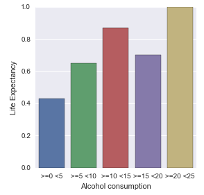
The analysis of this graph without other analysis (like the frequencies), maybe can lead an error. It seems to show that the most country with the life expectancy greater than the mean are those that alcohol consumption is in the range between 20 and 25 liters.
Graph of count observations
Is easy to see the equivocal examining the contigency table, on the column of category >=20 <25 we can verify that only one observation was collected. To help, even more, this issue, I used the countplot seaborn function, that is “A special case for the bar plot is when you want to show the number of observations in each category rather than computing a statistic for a second variable. This is similar to a histogram over a categorical, rather than quantitative, variable.”, Se here.

On this graph is easy to see that only 1 observation was realized in the column >=20 <=25.
Chi-Square
Chi-square calculations, wich include the chi-square value, the associated p-vale, and a table of expected counts that ares used in these calculations.
cs1 = scipy.stats.chi2_contingency(ct1)
results = OrderedDict()
results['chi-square'] = cs1[0]
results['p-value'] = cs1[1]
results['df'] = cs1[2]
print (tabulate([results.values()], tablefmt="fancy_grid",
                headers=[i for i in results.keys()]))
Code in section [282] on this notebook
| chi-square | p-value | df |
|---|---|---|
| 20.5031 | 0.000397211 | 4 |
Looking at the significant P value, we will accept the alternate Hypothesis, where not all life expectancy rates are equal across alcohol consumption categories. If my explanatory variable had only two levels, I could interpret the two corresponding column percentages and be able to say wich group had a significantly higher rate of life expectancy. But my explanatory variable has five categories. So I know that not all are equal. But I don’t know wich are different and wich are not.
Post Hoc Bonferroni Adjustment
On Bonferroni Adjustment p value had adjusted dividing p 0.05 by the number of comparisions that we plan to make
p_for_reject_h0 = .05/10

pairs = []
pairs.append((('>=0 <5','>=5 <10'),[0,5,5,10]))
pairs.append((('>=0 <5','>=10 <15'),[0,5,10,15]))
pairs.append((('>=0 <5','>=15 <20'),[0,5,15,20]))
pairs.append((('>=0 <5','>=20 <25'),[0,5,20,25]))
pairs.append((('>=5 <10','>=10 <15'),[5,10,10,15]))
pairs.append((('>=5 <10','>=15 <20'),[5,10,15,20]))
pairs.append((('>=5 <10','>=20 <25'),[5,10,20,25]))
pairs.append((('>=10 <15','>=15 <20'),[10,15,15,20]))
pairs.append((('>=10 <15','>=20 <25'),[10,15,20,25]))
pairs.append((('>=15 <20','>=20 <25'),[15,20,20,25]))

data_pairs = []
results=[]
for pair in pairs:
    data_pair = data2[ (((data1.alcohol>pair[1][0]) & (data1.alcohol<=pair[1][1])) |
                  ((data1.alcohol>pair[1][2]) & (data1.alcohol<=pair[1][3])))]

    ct0=pd.crosstab( data_pair['life'], data_pair['alcohol'])
    ct1 = ct0[ [pair[0][0],pair[0][1]] ]
    cs0 = scipy.stats.chi2_contingency(ct1)
    #print (ct0)

    # chi-square, p=value and degree of freedom
    reject = 'yes' if (cs0[1] < .05/10) else 'no'
    results.append((pair[0],cs0[0],cs0[1],cs0[2], reject))

print (tabulate(results, tablefmt="fancy_grid",
                headers=['groups', 'chi-square', 'p-value', 'df', 'h0 reject'] ))
Code in section [283] on this notebook
| groups | chi-square | p-value | df | h0 reject |
|---|---|---|---|---|
| (‘>=0 <5’, ‘>=5 <10’) | 5.53236 | 0.0186679 | 1 | no |
| (‘>=0 <5’, ‘>=10 <15’) | 15.773 | 7.14144e-05 | 1 | yes |
| (‘>=0 <5’, ‘>=15 <20’) | 1.64614 | 0.199485 | 1 | no |
| (‘>=0 <5’, ‘>=20 <25’) | 0.0169283 | 0.89648 | 1 | no |
| (‘>=5 <10’, ‘>=10 <15’) | 3.92657 | 0.0475288 | 1 | no |
| (‘>=5 <10’, ‘>=15 <20’) | 0.00235204 | 0.96132 | 1 | no |
| (‘>=5 <10’, ‘>=20 <25’) | 0.108449 | 0.741917 | 1 | no |
| (‘>=10 <15’, ‘>=15 <20’) | 0.586965 | 0.443595 | 1 | no |
| (‘>=10 <15’, ‘>=20 <25’) | 1.32719 | 0.249306 | 1 | no |
| (‘>=15 <20’, ‘>=20 <25’) | 0.286458 | 0.592499 | 1 | no |
Conclusion
Although in the first chi-square calculus the p-value indicated that the null hypothesis could be rejected (p-value < .05), the table above, resulting of Post hoc Bonferroni Adjustment, where the chi2 is calculated for all group each against each other (two by two), show us that the only comparison that we can reject the null hypothesis is >=0 <5 and >=10 <15 suggesting that if exists correlation between life expectancy and alcohol consumption is among the countries that have the levels of alcohol consumption between 0 and 5 and 10 and 15 liters.
See the entire code for this week here.