Now is the time in that we going to begin to visualize our variables with graphs. Though three or more variable could be selected, in the name of clarity and simplicity and for to focus on the hypothesis of the project , I opted for only 2: Life Expectancy and alcohol consumption. For more information about my project, click here. The entire code for this week can see here.

• Univariate histograms for quantitative variables
  • Univariate for alcohol
    • descriptive statistics
  • Univariate for life
    • descriptive statistics

The explanatory and response variables, life expectancy and alcohol consumption respectively, are quantitative, thus are presented in a scatter graph.

• Scatterplot

During the second week, I created the Categorical Variables and the respective Data dictionary (See here), Now the respectives bar graph is showing:

• Univariate bar graphs for categorical variables
  • Bar graph for life
  • Bar graph for alcohol

As the scatter graph had been a bit confused, I decided to convert one of the variable (the dependent) in categorical and then to plot the explanatory/response variable in a bar graph.

• Bivariate Bar Graph

Though this not a scientific work, I wrote a conclusion.

• Conclusion

Univariate histograms for quantitative variables

Univariate histogram for alcohol consumption:

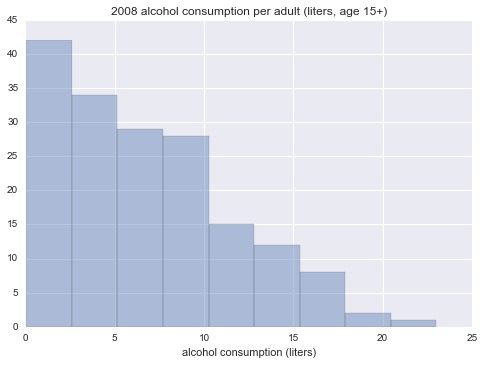
Standard deviation and other descriptive statistics for quantitative variable alcohol

╒═════════╤═════════╤═════════╤═══════╤═══════╤═══════╤═══════╤═══════╕
│   count │    mean │     std │   min │   25% │   50% │   75% │   max │
╞═════════╪═════════╪═════════╪═══════╪═══════╪═══════╪═══════╪═══════╡
│     171 │ 6.78409 │ 4.95145 │  0.05 │ 2.725 │  5.92 │  9.99 │ 23.01 │
╘═════════╧═════════╧═════════╧═══════╧═══════╧═══════╧═══════╧═══════╛

For code, see section [66] and [67] on this jupyter notebook..

Univariate histogram for life expectancy:

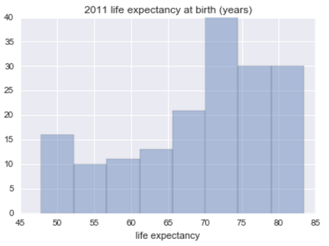
Standard deviation and other descriptive statistics for quantitative variable life.

╒═════════╤═════════╤═════════╤════════╤════════╤════════╤════════╤════════╕
│   count │    mean │     std │    min │    25% │    50% │    75% │    max │
╞═════════╪═════════╪═════════╪════════╪════════╪════════╪════════╪════════╡
│     171 │ 69.3857 │ 9.72824 │ 47.794 │ 62.747 │ 72.974 │ 76.099 │ 83.394 │
╘═════════╧═════════╧═════════╧════════╧════════╧════════╧════════╧════════╛

For code, see section [68] and [69] on this jupyter notebook.

Scatterplot for the association between Alcohol Consumption and Life Expectancy:

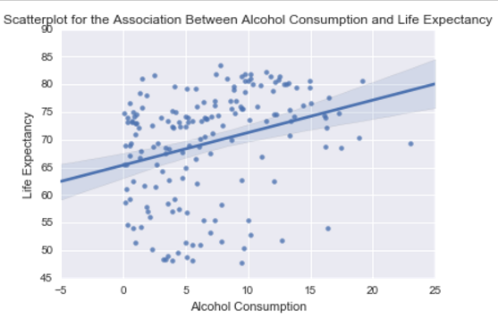
For code, see section [70] on this jupyter notebook.

Univariate bar graphs for categorical variables

Univariate bar graph for categorical variable life:

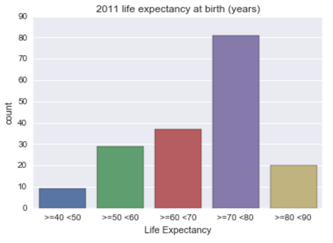
For code, see section [71] on this jupyter notebook.

univariate bar graph for categorical variable alcohol

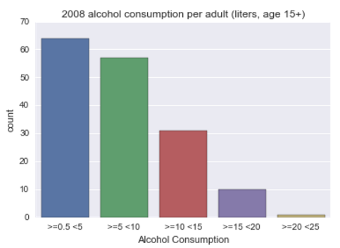
For code, see section [72] on this jupyter notebook.

Bivariate bar graph

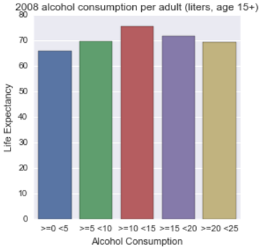
For code, see section [74] and this jupyter notebook.

Conclusion

Analysing only the scatter graph seems do not be a correlation between the variables, but considering the bivariate bar graph we can say that moderate alcohol consumption can contribute to life expectancy increases. Of course, this not a scientific work and have value only for this context.