Machine Learning and Data Analysis - Week2 | Random Forest
This is the second assignment of the fourth course (of five) Data Analysis and Interpretation Specialization detailed information about it can be seeing here.
See the entire code and output for this week, here.
This assignment deals with Lasso Regression Analysis that provides information for to obtain a subset of predictors that minimizes prediction error for a quantitative response variable.
Index
Variables
Details of my project can be seeing here, For this assignment, I add 10 variables, to get easier, I made a summary bellow:
|Variable Name|Description|Type|Kind|
|————-|———–|:———:|:—–:|:–:|
|Income |GPD per capita |C|E|
|Alcohol |Alcohol Consumption |C|E|
|Army |Armed force rate|Q|E|
|bCancer |Breast Cancer rate|Q|E|
|CO2 |Co2 emissions rate|Q|E|
|Female-employ|Female employ rate|Q|E|
|Net-rate |Internet users rate|Q|E|
|polity |Democracy indicator score|Q|E|
|relectricperperson| relectric per person|Q|E|
|suicide|Suicide per 100th|Q|E|
|Employ|Employment rate|Q|E|
|Urban|Urbanization rate|Q|E|
|Life |Life Expectancy|Q|R|
Type: C = Categorical, Q = Quantitative
Kind: E = Explanatory, R = Response
Coeficients
Data were randomly split into a training set that included 70% of the observations and a test set that included 30% of the observations. The least angle regression algorithm with k=10 fold cross validation was used to estimate the lasso regression model in the training set, and the model was validated using the test set. The change in the cross validation average (mean) squared error at each step was used to identify the best subset of predictor variables.
Bellow I shows de code an te table with coefficients generated
#select predictor variables and target variable as separate data sets
pred_cols = features
predvar = data1[pred_cols]

# standardize predictors to have mean=0 and sd=1
predictors=predvar.copy()
predictors = to_num(pred_cols, predictors)

target = data1.life

from sklearn import preprocessing

for p in [pred_cols]:
    predictors[p]=preprocessing.scale(predictors[p].astype('float64'))

# split data into train and test sets
pred_train, pred_test, tar_train, tar_test = train_test_split(predictors, target,
                                                              test_size=.3, random_state=123)

# specify the lasso regression model
model=LassoLarsCV(cv=10, precompute=False).fit(pred_train,tar_train)

# print variable names and regression coefficients
coefs = dict(zip(predictors.columns, model.coef_))

print(tabulate(pd.DataFrame(list(coefs.items())), tablefmt="grid", headers=['Variable', 'Coef']))
| Variable | Coef |
|---|---|
| female-employ | -1.31691 |
| employ | 0 |
| army | 0.815667 |
| suicideper100th | -0.71429 |
| relectricperperson | 0 |
| polity | 0.726064 |
| net-rate | 5.43781 |
| co2 | 1.1599 |
| urban | 0.821296 |
| alcohol | -0.0884026 |
| income | 0 |
| bcancer | 0.393847 |
As we can see from 12 explanatory variables, only six have coefficient greater than zero.
Conclusion
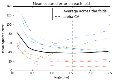
Of the 12 predictor variables, 6 were retained in the selected model. During the estimation process, the internet rate and co2 emissions were most strongly associated with life expectancy.
The explanatory variables were chosen randomly whose goal was only for this assignment. maybe, for this, probably there are details (like a lurking variable, for example.) that necessities a more deep study and analysis.
See the entire code and output for this week, here.