Machine Learning and Data Analysis - Week4 | K-Means
This is the fourth assignment of the fourth course (of five) Data Analysis and Interpretation Specialization detailed information about it can be seeing here.
See the entire code and output for this week, here.
This assignment deals with k-means cluster “Cluster analysis is an unsupervised machine learning method that partitions the observations in a data set into a smaller set of clusters where each observation belongs to only one cluster. The goal of cluster analysis is to group, or cluster, observations into subsets based on their similarity of responses on multiple variables.”
Index
- Variables
- Average Distance From Observations
- First Two Canonical Variables
- Cluster Differences In GPA Using ANOVA
Variables
Details of my project can be seeing here, For this assignment, I add 10 variables, to get easier, I made a summary bellow:
| Variable Name | Description | Type | Kind |
|---|---|---|---|
| Income | GPD per capita | C | E |
| Alcohol | Alcohol Consumption | C | E |
| Army | Armed force rate | Q | E |
| bCancer | Breast Cancer rate | Q | E |
| CO2 | Co2 emissions rate | Q | E |
| Female-employ | Female employ rate | Q | E |
| Net-rate | Internet users rate | Q | E |
| polity | Democracy indicator score | Q | E |
| relectricperperson | relectric per person | Q | E |
| suicide | Suicide per 100th | Q | E |
| Employ | Employment rate | Q | E |
| Urban | Urbanization rate | Q | E |
| Life | Life Expectancy | Q | R |
Type: C = Categorical, Q = Quantitative
Kind: E = Explanatory, R = Response
Average Distance From Observations
Data were randomly split into a training set that included 70% of the observations (N=84) and a test set that included 30% of the observations (N=36). A series of k-means cluster analyses were conducted on the training data specifying k=1-9 clusters, using Euclidean distance. The variance in the clustering variables that was accounted for by the clusters (r-square) was plotted for each of the nine cluster solutions in an elbow curve to provide guidance for choosing the number of clusters to interpret.
# k-means cluster analysis for 1-9 clusters
from scipy.spatial.distance import cdist
range_clusters=range(1,9)
meandist=[]

for k in range_clusters:
    model=KMeans(n_clusters=k)
    model.fit(clus_train)
    clusassign=model.predict(clus_train)
    meandist.append(sum(np.min(cdist(clus_train, model.cluster_centers_, 'euclidean'), axis=1))
    / clus_train.shape[0])

    plt.subplots(figsize=(12, 8))
    plt.plot(range_clusters, meandist)
    plt.xlabel('Number of clusters')
    plt.ylabel('Average distance')
    plt.title('Selecting k with the Elbow Method')

    plt.show()
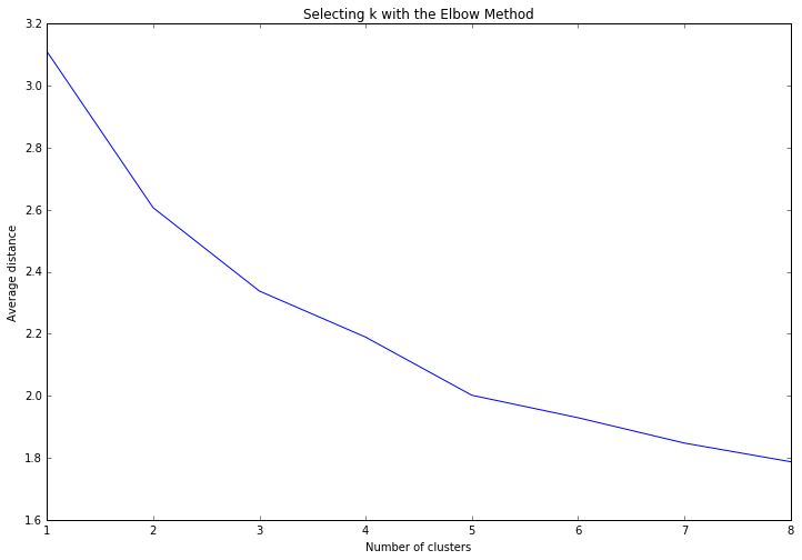
The elbow curve was inconclusive, suggesting that the 2, 3 and 5-cluster solutions might be interpreted. The results below are for an interpretation of the 3-cluster solution.
First Two Canonica Variables
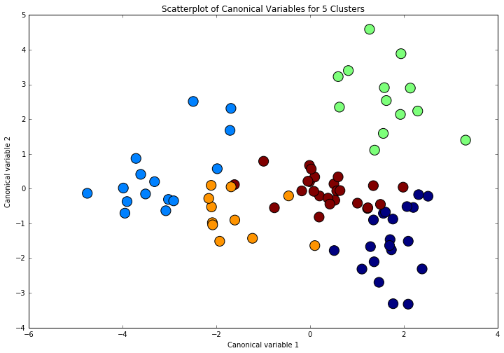
Canonical discriminant analyses was used to reduce the 12 clustering variable down a few variables that accounted for most of the variance in the clustering variables. A scatterplot of the first two canonical variables by cluster (Figure 2 shown below) indicated that the observations in clusters was generally distinct whith greater spread, suggesting higher within cluster variance.
Figure 2. Plot of the first two canonical variables for the clustering variables by cluster.
Cluster Differences In GPA Using ANOVA
In order to externally validate the clusters, an Analysis of Variance (ANOVA) was conducting to test for significant differences between the clusters on grade point average (GPA). A tukey test was used for post hoc comparisons between the clusters. Results indicated significant differences between the clusters on GPA. The tukey post hoc comparisons indicating null hypothesys rejection on comparisons between groups 0,1; 0,4; 1,2; 1,4; 2,4; 3,4 and 4,5.
gpa_data=data0['life']
# split GPA data into train and test sets
gpa_train, gpa_test = train_test_split(gpa_data, test_size=.3, random_state=123)
gpa_train1=pd.DataFrame(gpa_train)
gpa_train1.reset_index(level=0, inplace=True)
merged_train_all=pd.merge(gpa_train1, merged_train, on='index')
sub1 = merged_train_all[['life', 'cluster']].dropna()

import statsmodels.formula.api as smf
import statsmodels.stats.multicomp as multi

gpamod = smf.ols(formula='life ~ C(cluster)', data=sub1).fit()
print (gpamod.summary())

OLS Regression Results
==============================================================================
Dep. Variable:                   life   R-squared:                       0.529
Model:                            OLS   Adj. R-squared:                  0.505
Method:                 Least Squares   F-statistic:                     22.15
Date:                Sat, 12 Nov 2016   Prob (F-statistic):           2.73e-12
Time:                        14:57:59   Log-Likelihood:                -271.73
No. Observations:                  84   AIC:                             553.5
Df Residuals:                      79   BIC:                             565.6
Df Model:                           4
Covariance Type:            nonrobust
===================================================================================
coef    std err          t      P>|t|      [95.0% Conf. Int.]
-----------------------------------------------------------------------------------
Intercept          71.4555      1.758     40.646      0.000        67.956    74.955
C(cluster)[T.1]     0.5833      2.537      0.230      0.819        -4.467     5.634
C(cluster)[T.2]    -0.3662      2.183     -0.168      0.867        -4.711     3.979
C(cluster)[T.3]   -10.6704      2.258     -4.725      0.000       -15.165    -6.176
C(cluster)[T.4]     9.4513      2.402      3.935      0.000         4.670    14.232
==============================================================================
Omnibus:                       17.615   Durbin-Watson:                   2.144
Prob(Omnibus):                  0.000   Jarque-Bera (JB):               22.602
Skew:                          -0.982   Prob(JB):                     1.24e-05
Kurtosis:                       4.613   Cond. No.                         6.62
==============================================================================

mc1 = multi.MultiComparison(sub1['life'], sub1['cluster'])
res1 = mc1.tukeyhsd()
print(res1.summary())

Multiple Comparison of Means - Tukey HSD,FWER=0.05
==============================================
group1 group2 meandiff  lower    upper  reject
----------------------------------------------
  0      1     0.5833  -6.5008   7.6674 False
  0      2    -0.3662  -6.4602   5.7277 False
  0      3    -10.6704 -16.9748  -4.366  True
  0      4     9.4513   2.7457  16.1569  True
  1      2    -0.9495   -7.206   5.3069 False
  1      3    -11.2537 -17.7154  -4.792  True
  1      4     8.868    2.0143  15.7216  True
  2      3    -10.3041 -15.6619 -4.9464  True
  2      4     9.8175   3.993    15.642  True
  3      4    20.1217  14.0773   26.166  True
----------------------------------------------
See the entire code and output for this week, here.