Regression Modeling in Practice - Week2 | Basics of Linear Regression
This is the second assignment or the third course (of five) Data Analysis and Interpretation Specialization detailed information about it can be seeing here.
Index
Variables
Details of my project can be seeing here, to get easier,I made a summary bellow:
| Variable Name | Description | Type |
|---|---|---|
| Income | moderator: GPD per capita (1) | Explanatory Quantitative |
| Life | Explanatory Variable: Life Expectancy (2) | Response Quantitative |
(1) 2010 Gross Domestic Product per capita in constant 2000 US$”
(2) 2011 life expectancy at birth (years)
Center the Explanatory Variable
Though my explanatory variable is quantitative, there is much observation around zero value, even so, I center it to attend the requisites. the code bellow shows the procedure, first I calculated the mean and then a new variable (income_center) that represents the new values for var “income”, now with new mean.
# Measures for center and graph
measures = OrderedDict()
measures['Mean'] = data1.income.mean()

# New var for center the mean
data1['income_center'] = data1.income-measures['Mean']

measures['Center'] = data1.income_center.mean()
measures['cMin'] = data1.income_center.min()
measures['cMax'] = data1.income_center.max()
measures['Min life'] = data1.life.min()
measures['Max life'] = data1.life.max()

# Table shows measures
print (tabulate([measures], tablefmt='grid', headers='keys'))
| Mean | Center | cMin | cMax | Min life | Max life |
|---|---|---|---|---|---|
| 7327.44 | -1.1007e-12 | -7223.67 | 44974.1 | 47.794 | 83.394 |
This table shows the measures, Mean is the original mean and the center is the new mean, other measures (min and max of center, min and max of life) was calculated for help in graph plot.
For see the code, click here.
Summary
print ("OLS regression model")
reg1 = smf.ols('life ~ income', data=data1).fit()
print (reg1.summary())

OLS regression model
                            OLS Regression Results
==============================================================================
Dep. Variable:                   life   R-squared:                       0.362
Model:                            OLS   Adj. R-squared:                  0.358
Method:                 Least Squares   F-statistic:                     98.65
Date:                Sat, 24 Sep 2016   Prob (F-statistic):           1.07e-18
Time:                        13:57:02   Log-Likelihood:                -610.14
No. Observations:                 176   AIC:                             1224.
Df Residuals:                     174   BIC:                             1231.
Df Model:                           1
Covariance Type:            nonrobust
=================================================================================
                    coef    std err          t      P>|t|      [95.0% Conf. Int.]
---------------------------------------------------------------------------------
Intercept        69.6547      0.588    118.550      0.000        68.495    70.814
income_center     0.0006   5.58e-05      9.932      0.000         0.000     0.001
==============================================================================
Omnibus:                       19.382   Durbin-Watson:                   1.948
Prob(Omnibus):                  0.000   Jarque-Bera (JB):               23.222
Skew:                          -0.877   Prob(JB):                     9.06e-06
Kurtosis:                       2.698   Cond. No.                     1.05e+04
==============================================================================
The results of the linear regression model shows high F-statistic (98.05) and a very small p-value (1.07e-18), considerably less than our alpha level of 0.05. This indicated that life expectancy was significantly and positively associated with number level income.
The coefficient for income is 0.0006 ande the intercept is 65.5966. So now we know that our equation for the best fit line of this graph is:
life = 69.6547 + 0.0006 * income
The OLS regression results shows the R-Squared = 0.36 (The proprotion of the variance in the response variable that can be explained by the Explanatory variable), indicating that this model accounts for about 36% of the variability we see in response variable, life.
For see the code, click here.
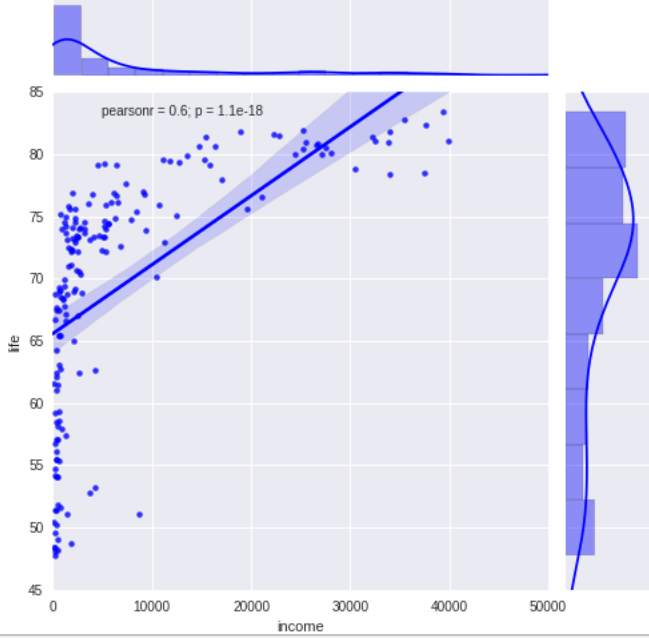
graph
See the entire code for this week, here.