Regression Modeling in Practice - Week3 | Multiple Regression
This is the third assignment or the third course (of five) Data Analysis and Interpretation Specialization detailed information about it can be seeing here.
Index
- Variables
- Sumary of OLS Results
- Support for hypothesis
- Evidence of confounding variable
- Regression Diagnostic
- OLS Output
Variables
Details of my project can be seeing here, to get easier, I made a summary bellow:
| Variable Name | Description |
|---|---|
| Income | Explanatory Variable: GPD per capita (1) |
| Alcohol | Explanatory Variable:: Alcohol Consumption (3) |
| Life | Response Variable: Life Expectancy (2) |
(1) 2010 Gross Domestic Product per capita in constant 2000 US$”
(2) 2011 life expectancy at birth (years)
(3) 2008 alcohol consumption per adult (liters, age 15+)
Sumary of OLS Results
The figure bellow represents part of OLS output of my Regression, for detail of variables see section Variables.
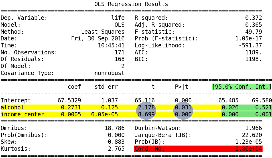
Examine the p values and parameter estimates for each predictor variable. IE the explanatory variable, alcohol, and the potential confounder, income. As we can see both P values are less than 0.05. And both of the parameter estimates are positive. Indicating that socioeconomic status and income levels have a direct correlation with the level of alcohol consumption of a country. For both, we can reject the null hypothesis.
Looking at the Confident intervals (highlighted in green) though we see that for the alcohol variable ranges from 0.026 to 0.521 meaning that we’re 95% certain that the true population parameter for the association between alcohol consumption levels and life expectancy fall somewhere between 0.026 and 0.521, and for the income variable betwen 0.00 and 0.01
Support for primary hypotheses
My primary hypothesis is “The level of alcohol consumption of a country might be directly related to expectancy life.”. After adding the variable income (income levels) is possible to note that results show the association between my primary explanatory and response variable.
In other words, alcohol is positively associated with the life expectancy after controlling for income levels. And, income level is positively associated with the life expectancy after controlling for the alcohol consumption levels.
Evidence of confounding variable.
Examining the output (the first without and the other with the income variable) is possible to note, through the big F-statistic and the Probability of F-statistic less than 0.05 that there is no evidence of confounding for the association between the primary explanatory and response variable.
Regression Diagnostic.
First I added a new explanatory variable, urban rate to my regression equation
see code in section 6 on this jupyter notebook. The intercept is the value of the response variable when all explanatory variables are held constant at zero. Because the two explanatory variables are centered , so that the mean for each variable was equal to zero, the intercept is the life expectancy at the mean of urban rate, and income level.
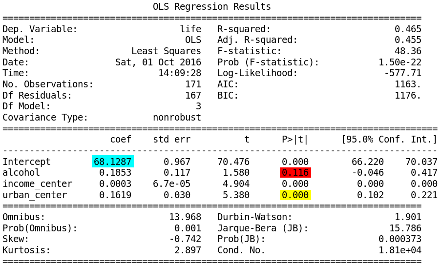
So the life expectancy when alcohol consumption and urban rate are at their means is 68,13% (highlighted in blue). There is also a show that the coefficients income variable remains significant after adjusting for urban rate (highlighted in yellow), but the alcohol variable become not statistically significant.
Qq Plot.
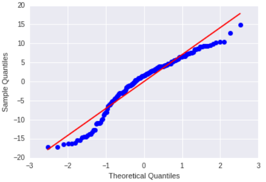
The qqplot for my regression model shows that the residuals generally follow a straight line, but deviate at the lower and higher quartiles. This indicates that the residuals did not follow a perfectly normal distribution.
Ploting Diagnostic.
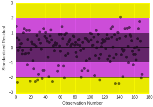
The plot of the standardized residuals shows us that 95% of the values of the residuals to fall between two standard deviations of the mean (the central highlighted area). So basically, they’re either between -1 or 1, and all but a few countries have residuals that are more than 2 standard deviations above or below the mean of 0 (the expanded central area). The residuals fall between two standard deviations of the mean.
Residual values that are more than two standard deviations from the mean in either direction (areas highlighted in yellow) are a warning sign that we may have some outliers.
Extreme outliers can not be observed since there is no deviation equal or greater than 3.
“If more than 1% of our observations has standardized residuals with an absolute value greater than 2.5, or more than 5% have an absolute value of greater than or equal to 2, then there is evidence that the level of error within our model is unacceptable. That is the model is a fairly poor fit to the observed data. None of the residuals from our value exceeded an absolute value of 2.5.” In this case, there are no absolutes values greater than 2.5 but there are 6,1% of values greater than or equal to 2 , this indicates that there is evidence that the level of error within the model is unacceptable. That is the model is a fairly poor fit to the observed data.
Additional Ploting Diagnostic.
 For this exercise, I chose the to test the correlation of income level in life
expectancy .
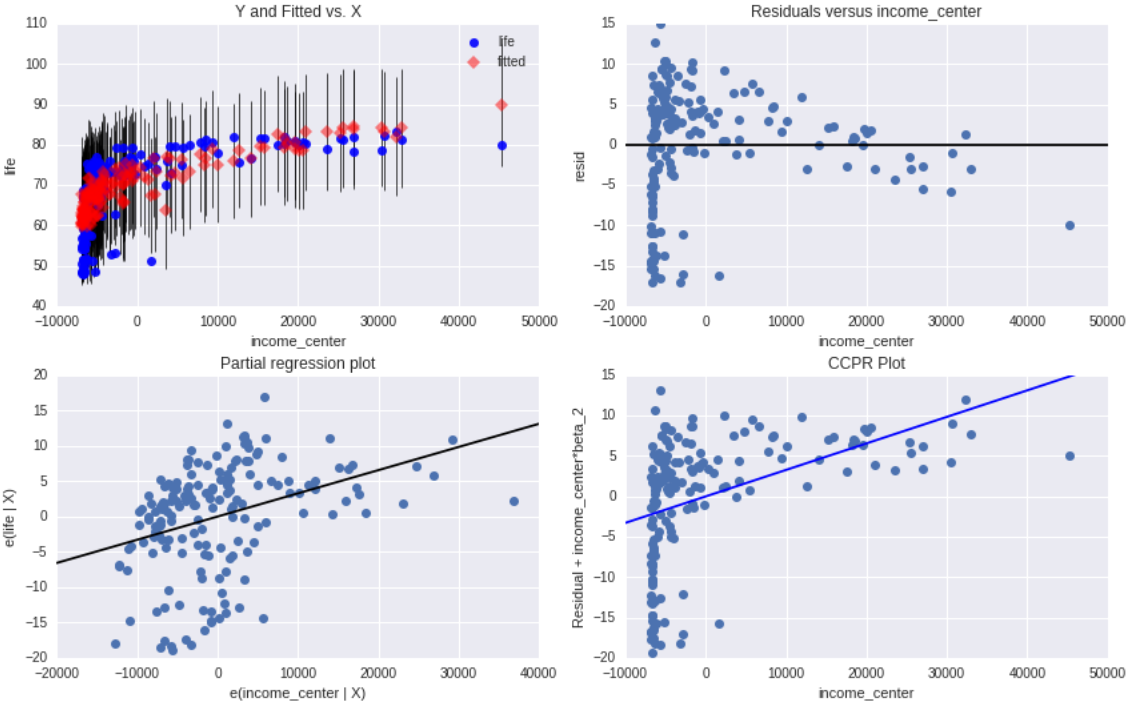
The plot in the upper right-hand corner shows the residuals for each observation at different values of income level.
Is easy to note that there are absolute values of the residuals significant larger and smaller at lower values of income level, but as income level increases the residuals values get smaller with only one large. this indicates that the as income increase the life expectancy too.
For this exercise, I chose the to test the correlation of income level in life
expectancy .
The plot in the upper right-hand corner shows the residuals for each observation at different values of income level.
Is easy to note that there are absolute values of the residuals significant larger and smaller at lower values of income level, but as income level increases the residuals values get smaller with only one large. this indicates that the as income increase the life expectancy too.
Leverage Plot.
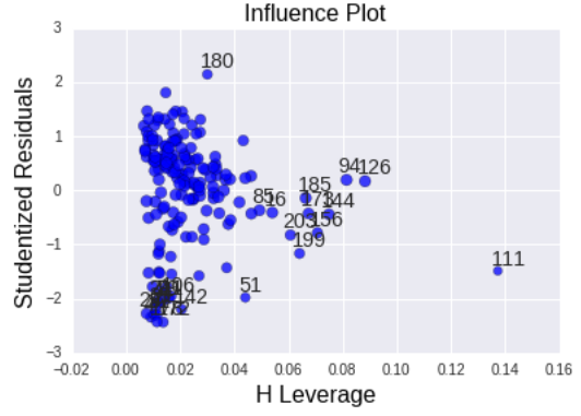
“A leverage plot to identify observations that have an unusually large influence on the estimation of the predicted value of the response variable, female employment rate, or that are outliers, or both. The leverage of an observation can be thought of in terms of how much the predicted scores for the other observations would differ if the observations in question were not included in the analysis. The leverage always takes on values between zero and one. A point with zero leverage has no effect on the regression model. And outliers are observations with residuals greater than 2 or less than -2.” In this laverage graph we can see that we have a few outliers, represented by the residuals greater than 2 and less than -2. but this plot also tells us that these outliers have small or close to zero leverage values, meaning that although they are outlying observations, they do not have an undue influence on the estimation of the regression model. On the other hand, we see that there are a only one case with higher than average leverage in terms of having an influence on the estimation of the predicted value of life expectancy. This observation has a high leverage but is not an outlier. We don’t have any observations that are both high leverage and outliers.
Output of OLS.
See the entire code and output for this week, here.