Regression Modeling in Practice - Week4 | Logistic Regression
This is the fourth assignment of the third course (of five) Data Analysis and Interpretation Specialization detailed information about it can be seeing here.
Index
- Variables
- Sumary of OLS Results
- Addin income variable
- Evidence of confounding variable
- OLS Output
- Certificate
Variables
Details of my project can be seeing here, to get easier, I made a summary bellow:
| Variable Name | Description |
|---|---|
| Income | Explanatory Variable: GPD per capita (1) |
| Alcohol | Explanatory Variable:: Alcohol Consumption (3) |
| Life | Response Variable: Life Expectancy (2) |
(1) 2010 Gross Domestic Product per capita in constant 2000 US$”
(2) 2011 life expectancy at birth (years)
(3) 2008 alcohol consumption per adult (liters, age 15+)
Sumary of OLS Results
The figure bellow represents part of OLS output of my Regression, for detail of variables see section Variables. First I selected only 2 variables for the initial analysis, later I added another for analysis of confounder.
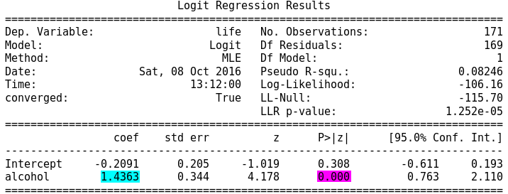
The regression is significant at a P value of less than 0.0001 (highlighted in red), using parameters estimated, the linear equation can be generated: Life expectancy is a function of -0.21 plus 1.44 times alcohol, but with the logistic regression is appropriated to use odds ratio.
Support hypothesis
Before we analyse the Odds ratio, we can conclude, through these initial results, that socioeconomic have a direct correlation with the level of alcohol consumption of a country. Then, we can reject the null hypothesis.
Odds Ratio and Confidence intervals
params = lreg1.params
conf = lreg1.conf_int()
conf['OR'] = params
conf.columns = ['Lower CI', 'Upper CI', 'OR']

print (np.exp(conf))

           Lower CI  Upper CI       OR
Intercept  0.542615  1.213092 0.811321
alcohol    2.143658  8.249307 4.205198
The Odds ratios indicate that there’s 95% certainty that two parameters odd ratio fall between 2.14 and 8.25, that is, the alcohol consumption above the mean (6.8 liters per year) represents a life expectancy above the mean (69 years) something anywhere from 2.14 to 8.2 times more likely than those countries that have alcohol consumption levels less than the mean.
Adding Income Variable
Here I added the income levels variabe (see section Variables), for the secoond analysis (see code for this in section [13] on this notebok
New Summary OLS results
The figure bellow represent the OLS results after I added the income levels.
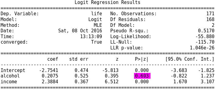
Evidence of Confounding
Looking at the news results is possible to note that the inclusion of the new variable (income) change the alcohol p value (highlighted in red), this indicates the evidence of confounding.
Output of OLS.
See the entire code and output for this week, here.