This is the first assignment of the fourth course (of five) Data Analysis and Interpretation Specialization detailed information about it can be seeing here.

Index

• Variables
• Confusion Matrix
• Decision Tree
• Conclusion

Variables

Details of my project can be seeing here, to get easier, I made a summary bellow:

Variable Name	Description
Income	Explanatory Variable: GPD per capita (1)
Alcohol	Explanatory Variable:: Alcohol Consumption (3)
Life	Response Variable: Life Expectancy (2)

(1) 2010 Gross Domestic Product per capita in constant 2000 US$”

(2) 2011 life expectancy at birth (years)

(3) 2008 alcohol consumption per adult (liters, age 15+)

Confusion Matrix

The figure bellow represents the confusion matrix, for see the code that generated the matrix and this graph, visite the section 10 of this notebook

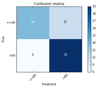
This graph represents the confusion matrix, that shows the correct and incorrect classifications of the decision tree, the labels means the life expectancy greater and less than 69 years, the horizontal labels are the predictions and the vertical are the reference (true). the main diagonal: 18 and 33 represent the number of true negative and true positive for life expectancy and the other diagonal (values 6 and 12) represents the numbers of false negative and false positive respectively.

Decison Tree

For this graph I used the parameters of tree.export_graphviz in this example For the code that generated this graph see the section [12] on this jupyter notebook

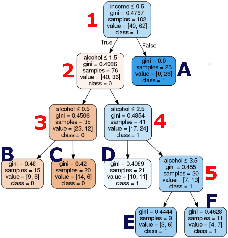
Here, the target is the life (my binary categorical variable) and alcohol consumption and income levels as the predictor or explanatory variables. The result tree starts with the split on income variable, my second explanatory variable. This binary variable has values of zero (0) representing income level less than or equals the mean (US$ 7.006,00) and value one (1) representing income greater than the mean. The resulting tree starts with the split on income variable. In the first split (1) we can see that 26 countries have the life expectancy and income levels greater than the mean (A) and the other 76 countries have the life expectancy less than the mean. The second split (2), splits in the other 2 internal nodes according to consumption alcohol levels and so on.

Through internal nodes 2, 4 and 5 and the leaves D, E, and F, we can see that the majority of countries with the life expectancy greater than the mean (Class 1) has the alcohol consumption between 2.5 and 3.5 liters per year (11 countries in leaf D)

Conclusion

It is easy to note the significance of the variable income. In the first split, we see that all countries that have income level greater than 0.5 (The mean) have the life expectancy greater than the mean (A - Blue leaf), independently of the consumption alcohol level. In the other hand, although the differences are subtle we can see than the among the countries that have income levels less than the mean, those that have alcohol consumption between 2.5 and 3.5 have the life expectancy greater than the mean.

See the entire code and output for this week, here.